Work in Progress

This document is still under development and may change frequently.

Time-Domain Magnetic Material

Introduction 

A time-domain magnetic material is defined by its magnetic permeability \(\mu\), electrical conductivity \(\sigma\), and magnetization properties \(\mathbf{M}\), with an additional flag to indicate if eddy currents are present. While a simplified approach is available to specify common materials presented here presented here, the user can define their own materials by specifying the material properties methods individually using:

my_material = TimeDomainMagneticGeneralMaterial(name="My Material",
                                                marker=my_material_marker,
                                                permeability_method=my_permeability_method,
                                                conductivity_method=my_conductivity_method,
                                                magnetization_method=my_magnetization_method,
                                                has_eddy_currents=True)

Where each of the three material properties ( \(\mu\), \(\sigma\), and \(\mathbf{M}\)) can be defined by specifying a property method to compute those.

Predefined materials are available for common materials, such as vacuum, copper, and iron using following functions.

Material Properties 

Magnetic Permeability 

In general, we distinguish between paramagnetic, diamagnetic, and ferromagnetic materials based on their response to an external magnetic field.

This table summarizes the relative permeability of some common materials.
Material	Type	Relative Permeability ( mu_r )
Aluminum	Paramagnetic	~1.00002
Tungsten	Paramagnetic	~1.0001
Oxygen (gas)	Paramagnetic	~1.000004
Copper	Diamagnetic	~0.999991
Gold	Diamagnetic	~0.99998
Carbon (graphite)	Diamagnetic	~0.9999995
Iron	Ferromagnetic	200 - 5000
Steel	Ferromagnetic	~2000
Nickel	Ferromagnetic	~600
Cobalt	Ferromagnetic	~250

While paramagnetic materials have a relative permeability slightly larger than 1, diamagnetic materials have a relative permeability slightly smaller than 1, and ferromagnetic materials have a relative permeability much larger than 1.

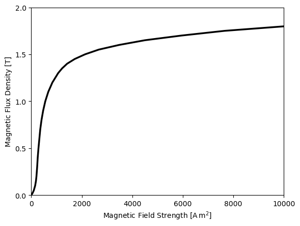
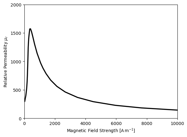
Ferromagnetic materials have a large permeability due to the alignment of magnetic moments in the material, which can be influenced by an external magnetic field. This effect is called magnetization; however for large fields the material may become saturated and the permeability may decrease. This behavior is described by a BH-curve.


A BH-curve from a ferromagnetic material. The magnetic flux density \(B\) is plotted against the magnetic field strength \(H\). A BH-curve is strictly monotonic. The slope of the curve is the magnetic permeability \(\mu\) of the material.

Once the material is saturated, the magnetic permeability falls back towards the vacuum permeability \(\mu_0\) for \(H \rightarrow \infty\).

In general the magnetic permeability is described by a symmetric two-rank tensor:

\[\begin{split}\begin{alignat}{2} \mu &= \left( \begin{array}{ccc} \mu_{xx} & \mu_{xy} & \mu_{xz} \\ & \mu_{yy} & \mu_{yz} \\ & & \mu_{zz} \end{array} \right) \end{alignat}\end{split}\]

Note that each component may additionally have dependency on other physical quantities, such as temperature or be nonlinear (dependent on the magnetic flux density).

The magnetic permeability can be defined by the following methods:

Magnetic Permeability Methods
Name	Description
Non Magnetic	the class MagneticPermeabilityMethodNonMagnetic gives \[\begin{align} \mu &= \mu_0 \mathbf{I} \quad, \end{align}\] specifies the magnetic permeability of the material to be vacuum permeability \(\mu_0\). Best used for materials that are paramagnetic or diamagnetic such as non-magnetic materials such as aluminum, copper or gases, or fluids.
Linear Isotropic	MagneticPermeabilityMethodLinearIsotropic \[\begin{align} \mu &= \mu_{\text{usr}}\mu_0 \mathbf{I} \quad, \end{align}\] specifies the relative magnetic permeability of the material to be a constant value \(\mu_{\text{usr}}\). Best used for magnetic material such as iron, steel, nickel, cobalt below saturation.
Nonlinear Isotropic	MagneticPermeabilityMethodNonlinearIsotropic \[\begin{align} \mu &= \mu(\|\mathbf{B}\|)_{\text{usr}} \mathbf{I} \quad, \end{align}\] specifies the magnetic permeability through a tabulated values of \(B\) and \(H\) (so called BH-curve).
Linear Anisotropic	MagneticPermeabilityPropertyMethodConstantTensor \[\begin{split}\begin{alignat}{2} \mu &= \left( \begin{array}{ccc} \mu_{xx} & \mu_{xy} & \mu_{xz} \\ & \mu_{yy} & \mu_{yz} \\ & & \mu_{zz} \end{array} \right) \end{alignat}\end{split}\] allows the specification of each individual component of the magnetic permeability tensor.

Electrical Conductivity 

The electrical conductivity is the measure of a material’s ability to conduct electric current. It is represented by the symbol \(\sigma\) (sigma) and is expressed in units of siemens per meter (S/m). Materials are categorized based on their conductivity into conductors (e.g., metals), insulators (e.g., glass), semiconductors (e.g., silicon), electrolytes (e.g., saltwater), and plasmas (e.g., ionized gases).

Electrical Conductivity of Materials
Material	Type	Electrical Conductivity \(\sigma \left[\frac{S}{m} \right]\)
Silver	Metal	\(6.30 \times 10^7\)
Copper	Metal	\(5.96 \times 10^7\)
Aluminum	Metal	\(3.50 \times 10^7\)
Iron	Metal	\(1.00 \times 10^7\)
Mercury	Liquid Metal	\(1.04 \times 10^6\)
Molten Sodium	Liquid Metal	\(2.10 \times 10^6\)
Glass	Insulator	\(10^{-11} \, \text{to} \, 10^{-15}\)
Rubber	Insulator	\(10^{-13}\)
Silicon	Semiconductor	\(10^{-4} \, \text{to} \, 10^{-1}\)
Saltwater	Electrolyte	\(1 \, \text{to} \, 10\)
Plasma (ionized gas)	Plasma	\(10^3 \, \text{to} \, 10^8\)
PEDOT:PSS	Conductive Polymer	\(10^2 \, \text{to} \, 10^4\)

In general, the electrical conductivity is described by a symmetric two-rank tensor:

\[\begin{split}\begin{alignat}{2} \sigma &= \left( \begin{array}{ccc} \sigma_{xx} & \sigma_{xy} & \sigma_{xz} \\ & \sigma_{yy} & \sigma_{yz} \\ & & \sigma_{zz} \end{array} \right) \end{alignat}\end{split}\]

Note that each component may additionally have dependency on other physical quantities, such as temperature or be nonlinear (dependent on the magnetic flux density). In many cases an isotropic material is assumed, where the tensor is diagonal.

Electrical Conductivity Methods
Name	Description
Insulating	ElectricConductivityPropertyMethodInsulating \[\begin{align} \sigma &= 0 \quad, \end{align}\] specifies the electrical conductivity of the material to be zero.
Constant	ElectricConductivityPropertyMethodConstant \[\begin{align} \sigma &= \sigma_{\text{usr}} \quad, \end{align}\] specifies the electrical conductivity of the material to be a constant value \(\sigma_{\text{usr}}\).
Constant Anisotropic	ElectricConductivityPropertyMethodConstantTensor \[\begin{split}\begin{alignat}{2} \sigma &= \left( \begin{array}{ccc} \sigma_{xx} & \sigma_{xy} & \sigma_{xz} \\ & \sigma_{yy} & \sigma_{yz} \\ & & \sigma_{zz} \end{array} \right) \end{alignat}\end{split}\] allows the specification of each individual component of the electrical conductivity tensor.
Constant Linear Temperature	ElectricConductivityMethodLinearTemperatureDependence \[\begin{align} \sigma &= \left( \sigma_{\text{ref}} - \gamma \left( T - T_{\text{ref}} \right) \right) \mathbf{I} \quad, \end{align}\] specifies the electrical conductivity of the material to be linearly dependent on the temperature. Here, \(\sigma_{\text{ref}}\) is the conductivity at the reference temperature \(T_{\text{ref}}\) and \(\gamma\) is the temperature coefficient of the material. Note that this requires a Temperature Model to be present.
Constant Temperature Table	ElectricConductivityMethodTemperatureTable \[\begin{align} \sigma &= \sigma(T) \mathbf{I} \quad, \end{align}\] specifies the electrical conductivity of the material to be a tabulated value dependent on temperature \(T\). Note that this requires a Temperature Model to be present.

Magnetization 

The remanence flux density, \(\mathbf{B}_r\), is a fundamental property of permanent magnets that describes the magnetic flux density retained in a material when the external magnetizing field is removed. It is closely related to the magnetization \(\mathbf{M}\), which represents the material’s magnetic moment per unit volume.

Some properties of common permanent magnets:

Magnet Type	Remanence \(\mathbf{B}_r[T]\)	Relative Permeability \(\mu_r[1]\)
Neodymium-Iron-Boron (NdFeB)	1.0 - 1.4	1.05 - 1.2
Samarium-Cobalt (SmCo)	0.8 - 1.2	1.05 - 1.15
Alnico	0.6 - 1.35	4 - 10
Ferrite (Ceramic)	0.2 - 0.45	1.05 - 1.1
Flexible Magnets	0.05 - 0.1	~1.05

There is a large variety in the remanence flux density and relative permeability of permanent magnets, depending on the material composition and manufacturing process as well as how temperature and external fields affect the magnetization.

The remanence flux density is described as a vector:

\[\mathbf{B}_r = B_r \mathbf{d} \quad,\]

where \(B_r\) is the remanence flux density and \(\mathbf{d}\) is the magnetization direction unit vector.

The magnetization can be defined by the following methods:

Magnetization Methods
Name	Description
Zero	MagnetizationPropertyMethodZero \[\begin{align} \mathbf{B}_r &= 0 \quad, \end{align}\] specifies the magnetization of the material to be zero.
Constant	MagnetizationPropertyMethodConstant \[\begin{align} \mathbf{B}_r &= \mathbf{B}_{r,\text{usr}} \quad, \end{align}\]

Examples 

We can create a linear permanent magnet material through a function using

from mufem.electromagnetics.timedomainmagnetic import TimeDomainMagneticGeneralMaterial


magnet_material = TimeDomainMagneticGeneralMaterial.Magnet(
          "Magnet Material",
          my_magnet_material_marker,
          relative_permeability=1.12,
          electric_conductivity=0.0,
          magnetization=[1.02, 0.0, 0.0],
)

the same can be achieved by specifying the methods individually using

from mufem.electromagnetics.timedomainmagnetic import (
  ElectricConductivityMethodInsulating,
  TimeDomainMagneticGeneralMaterial,
  MagneticPermeabilityMethodLinearIsotropic,
  MagnetizationMethodDirection
)

permeability_non_magnetic = MagneticPermeabilityMethodLinearIsotropic(1.12)
conductivity_insulating = ElectricConductivityMethodInsulating()
magnetization_direction = MagnetizationMethodDirection(1.02, 0.0, 0.0)

magnet_material = TimeDomainMagneticGeneralMaterial(
          "Magnet Material",
          my_magnet_material_marker,
          permeability_non_magnetic,
          conductivity_insulating,
          magnetization_direction,
)

Time-Domain Magnetic Material

Introduction

Material Properties

Magnetic Permeability

Electrical Conductivity

Magnetization

Examples