Time-Domain Magnetic Model

This model uses the quasi-static approximation of Maxwell’s equations where wave and displacement effects are neglected. This model is usually used to model low-frequency applications, where magnetic fields and eddy currents are dominating, such as in electric machines, transformers, and induction heating.

The model here uses the so-called A-formulation (also known as electric formulation), where we are solving for the magnetic vector potential \(\mathbf{A}\), given by:

(1)\[ \operatorname{curl} \nu \operatorname{curl} \mathbf{A} + \sigma \frac{\partial \mathbf{A}}{\partial t} = \mathbf{J} + \nu \operatorname{curl} \mathbf{B}_r \quad,\]

where:

\(\nu\) is the rank-2 magnetic reluctivity tensor,
\(\sigma\) is the rank-2 electrical conductivity tensor,
\(\mathbf{J}\) is a prescribed divergence-free current density (\(\operatorname{div} \mathbf{J}= 0\)),
\(\mathbf{B}_r\) is the remanent flux density.

Note that the magnetic flux density is related to the magnetic vector potential by:

\[\mathbf{B} = \operatorname{curl} \mathbf{A} \quad,\]

The magnetic reluctivity is the inverse of the magnetic permeability tensor (\(\nu = \mu^{-1}\)). The electric conductivity tensor \(\sigma\) is usually a diagonal tensor, where the off-diagonal terms are zero. It describes how well a material conducts electric current. The remanent flux density is related to the remanent magnetization (\(\mathbf{M}_r\)) by \(\mathbf{B}_r = \mu \mathbf{M}_r\).

Eq. (1) is augmented by the constitutive equations:

\[\begin{split}\begin{alignat}{2} \mathbf{H} &= \nu \left( \mathbf{B} - \mathbf{B}_r \right) &\quad, \\ \mathbf{J} &= \sigma \mathbf{E} &\quad, \end{alignat}\end{split}\]

Note that in general the material properties: \(\nu\), \(\sigma\), and \(\mathbf{M}\) can be nonlinear and dependent on other physical properties such as temperature.

In Eq. (1), the prescribed current density \(\mathbf{J}\) on the right-hand side is set through support models such as the Excitation Coil model.

Materials

The model (1) requires the provision of material properties, specifically the magnetic reluctivity (inverse permeability), the electrical conductivity and the magnetization. A material is created by specifying methods to compute each of those three material properties. For more details about materials, please see Time-Domain Magnetic Material.

To simplify the setup for common materials, we provide a setup function for common materials, such as vacuum, copper, and iron using following functions.

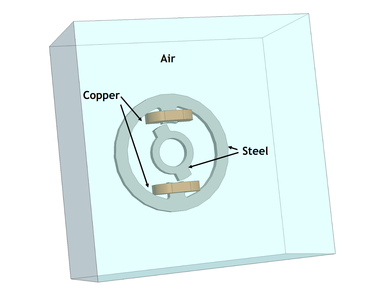
An example of showing a simulation with three materials: Air, Copper and Steel.

Predefined time-domain magnetic materials
Name	Description
Vacuum	Creates a vacuum material with \[\begin{split}\begin{alignat}{2} \mu &= \mu_0 &\quad, \\ \sigma &= 0 &\quad, \\ \mathbf{M} &= 0 &\quad, \end{alignat}\end{split}\] where \(\mu_0 \approx 4 \pi \times 10^{-7}\) is the vacuum permeability. This material can be used for air or vacuum, but also for insulators like plastics, ceramics or glass.
Non-Magnetic	Creates a non magnetic material with vacuum permeability, specified electric conductivity and no magnetization. \[\begin{split}\begin{alignat}{2} \mu &= \mu_0 &\quad, \\ \sigma &= \sigma_{\textrm{usr}} &\quad, \\ \mathbf{M} &= 0 &\quad, \end{alignat}\end{split}\] Can be used to model non-magnetic but conductive materials, where \(\sigma_{\textrm{usr}}\) is the electrical conductivity of the material specified by the user. This material can be used for metals like copper or aluminum, but also for conductive liquids like salt water.
Magnetic	Creates a magnetic material with non-vacuum permeability, specified electric conductivity and no magnetization. \[\begin{split}\begin{alignat}{2} \mu &= \mu_{\text{usr}} &\quad, \\ \sigma &= \sigma_{\text{usr}} &\quad, \\ \mathbf{M} &= 0 &\quad, \end{alignat}\end{split}\] Can be used to model magnetic materials like iron, cobalt or nickel when non-linear effects are not important where \(\mu_{\text{usr}}\) is the magnetic permeability and \(\sigma_{\text{usr}}\) is the electrical conductivity of the material specified by the user.
Non-Linear Magnetic	Creates a non-linear magnetic material with a constant electrical conductivity. \[\begin{split}\begin{alignat}{2} \mu &= \mu(\|\mathbf{B}\|)_{\text{usr}} &\quad, \\ \sigma &= \sigma_{\text{usr}} &\quad, \\ \mathbf{M} &= 0 &\quad, \end{alignat}\end{split}\] Can be used to model magnetic materials like iron or steel when non-linear effects are important, where \(\mu(\|\mathbf{B}\|)_{\text{usr}}\) is the non-linear magnetic permeability of the material and \(\sigma_{\text{usr}}\) is the electrical conductivity of the material specified by the user. In general a bh curve needs to be provided to define the non-linear magnetic properties.
Magnet	Creates a linear magnet \[\begin{split}\begin{alignat}{2} \mu &= \mu_{\text{usr}} &\quad, \\ \sigma &= \sigma_{\text{usr}} &\quad, \\ \mathbf{M} &= \mathbf{M}_{\text{usr}} &\quad, \end{alignat}\end{split}\] Can be used to model permanent magnets like neodymium or ferrite magnets where \(\mu_{\text{usr}}\) is the magnetic permeability of the material and \(\sigma_{\text{usr}}\) is the electric conductivity of the material and \(\mathbf{M}_{\text{usr}}\) is the constant magnetization of the material specified by the user.

Anisotropic materials can be defined by specifying the permeability tensor and the conductivity tensor, see Time-Domain Magnetic Material for more details.

More complex materials like hysteric, laminated and superconducting materials are supported in their respective modules.

Conditions

Following conditions are available for the time-domain magnetic model:

List of supported conditions
Name	Type	Description
Tangential Magnetic Flux	Boundary Condition	As boundary conditions, we support the tangential magnetic flux given by: \[\mathbf{n} \cdot \mathbf{B} = 0 \quad \text{on} \quad \Gamma_0,\] on the boundary \(\Gamma_0\).
Normal Magnetic Field	Boundary Condition	The normal magnetic field given by: \[\left. \mathbf{H} \times \mathbf{n} \right\|_{\Gamma_0} = 0 \quad,\]
Tangential Magnetic Field	Boundary Condition	The tangential magnetic field given by: \[\left. \mathbf{H} \times \mathbf{n} \right\|_{\Gamma_0} = \mathbf{H}_{\text{usr}} \quad,\] where \(\mathbf{H}_{\text{usr}}\) is the user-defined external magnetic field imposed on the boundary \(\Gamma_0\).

Reports

Following reports are available for the time-domain magnetic model for visualization:

List of reports
Name	Type	Description
Magnetic Force Report	Scalar Field	Returns the magnetic force density on an object
Magnetic Torque Report	Scalar Field	Returns the magnetic force density on an object

Coefficient Functions

Following functions are available for the time-domain magnetic model for visualization or querying:

List of functions
Name	Type	Description
Relative Magnetic Permeability	Scalar Field	The relative permeability is defined as: \[\mu_r = \frac{1}{3 \mu_0} \frac{1}{\operatorname{tr}\left( \bar{\bar{\nu}} \right)},\] where \(\operatorname{tr}\) is the trace operator and \(\mu_0\) is the vacuum permeability.
Magnetic Flux Density	Vector Field	The magnetic flux density is computed as: \[\mathbf{B} = \mathbf{\nabla} \times \mathbf{A}.\]
Magnetic Field	Vector Field	The magnetic field is given by: \[\mathbf{H} = \bar{\bar{\nu}} \mathbf{B} - \mathbf{H}_c,\] where \(\mathbf{H}_c\) is the coercive force.
Magnetic Energy Density	Scalar Field	The magnetic energy density is defined as: \[\epsilon = \int_{0}^{\|\mathbf{B}\|} \mathbf{H} \cdot \mathbf{B} \, \mathrm{d}B.\]
Electromechanical Stress Tensor	Tensor Field	The stress tensor is expressed as: \[\bar{\bar{\sigma}}_{\mathrm{em}} = \mathbf{H} \otimes \mathbf{B} - \frac{1}{2} \left( \mathbf{H} \cdot \mathbf{B} \right) \mathbb{I},\] where \(\mathbb{I}\) is the \(3 \times 3\) identity matrix.
Ohmic Heating	Scalar Field	The ohmic heating is computed as: \[P_\Omega = \mathbf{J} \cdot \mathbf{E}.\]
Lorentz Force Density	Vector Field	The Lorentz force density is given by: \[\mathbf{F}_L = \mathbf{J} \times \mathbf{B}.\]